Decoding in LLMs

A Deep Dive into the Linguistic Prowess of Large Language Models and Their Advanced Decoding Techniques 💥

There are lot of small technical pieces that come together to make the LLMs work the way they do. This sometimes feels like magic. 😀

There are different strategies which are employed while generating outputs from these LLMs. Different strategies suit different kinds of use cases. While I would not be able to cover all the proposed methods, I’ll be covering which I have been reading upon. Maybe others in another post.

So, the LLMs. We know that the transformer architecture sits at the core of this Language Model revolution. There have been other architectures proposed in recent times like SSM(e.g. MAMBA) but it is the transformers doing the heavy lifting as of now.

Loosely speaking, Transformer architecture has two sub-parts: Encoder and Decoder. Encoder takes the input data, encodes it into some intermediate representation, passes the representation to the decoder. The decoder then consumes the representations from the encoder, merges it with representations from its own input layers and then generates output, one token at a time. This ‘one token at each time step t_n, based on tokens generated from t₀ to t_n-1’ is called auto-regressive language modelling.

Majority, if not all, of the LLM in news recently use only the decoder part of the transformers. This means they let go of the encoder completely and all the connection from encoder flowing into decoder.

When generating an output token at timestep t, LLMs follow a three-step process:

1. Calculate output scores for each token in the vocabulary. This is called logits.

2. Convert logits to softmax scores, which gives us a probability distribution over the set of all tokens in the vocabulary.

3. Sample token(s) from this probability distribution as the output at time step t.

The 3^rd step above can follow varying strategies to condition the nature of output.

These strategies can be broadly divided into two classes: deterministic and stochastic. Each suits different task categories. For example, a close-ended task like classification should work well with deterministic methods while stochastic methods should favor open-ended tasks like creative writing. We will browse through each, while going deeper into some of them which are more frequently used.

This is the list we’ll follow:

Deterministic Strategies:

• Greedy Approach

• Beam Search (and Diverse Beam Search)

• Contrastive Decoding

• Contrastive Search

Stochastic Strategies:

• top-k sampling

• top-p sampling

• temperature based sampling

There are strategies which do not really change the quality/nature of the output but rather help improve the latency for token generation. Speculative Decoding is one such very interesting approach and is used widely to speed up the generation process. While it is not part of this post, it is a very interesting idea. Refer these papers to read about it.

• Accelerating Large Language Model Decoding with Speculative Sampling

• Fast Inference from Transformers via Speculative Decoding

Greedy Approach:

This is the simplest approach: just take the token with highest probability as the next output token.

\(\hat{y_t} = argmax\, P(y_t=v|y_{<t})\, \forall\, v \in V\)

Here V is the vocabulary set. This says, pick the token which has the highest probability, as predicted by the LLM, to be the output token at time t given all the tokens at time <t.

This method may suit close ended tasks like MT, summarization etc. When used for open ended generations like story writing, the model starts producing repetitive tokens and loses coherence as well.

Here is an example generation using GPT-2 model with the prompt “The city of delhi is”:

The city of delhi is a city of people, and the people of delhi are people of the world.

The city of delhi is a city of people, and the people of delhi are people of the world.

The city of delhi is a city of people, and the people of delhi are people of the world.

The city of delhi is a city of people, and the people of delhi are people of the world.

The city of delhi is a city of people, and the people of delhi are people of the world.

Beam Search:

With greedy search, we consider only a single token as output at each timestep t. That selection will impact every future token selection. The sequence that we end up, after greedy search has finished decoding, could have been different had we selected a different token at a certain time step.

Beam search allows us to select a probabilistically better sequence, rather than just focusing on the probabilistically best token at each time step. It does so by producing 'B' alternative sequences from each of the previous candidate sequence at a time step. Then at from all the generations at that time step, it selects ‘B’ tokens with the highest probability and moves forward. At the end of all the generations, we pick the sequence with the highest probability overall. The parameter 'B' is called beam width and controls how many alternatives are considered at each timestep.

By considering 'B' alternatives at each time step, beam search constructs a tree like structure. Once the sequence generation process is complete, it picks the path in the tree (each path represents one sequence) which has the highest combined probability.

For example, if the beam width is 3, that would mean at each timestep, beam search will consider the 3 best sequences so far, across all generations, and then proceed along those 3 sequences for further generation.

A quick example. Let’s assume we have a vocabulary set of all upper-case alphabets [A-Z]. Our beam width is 3. We start with a '<START>' token at time step T0.

Figure 1. Example of beam search

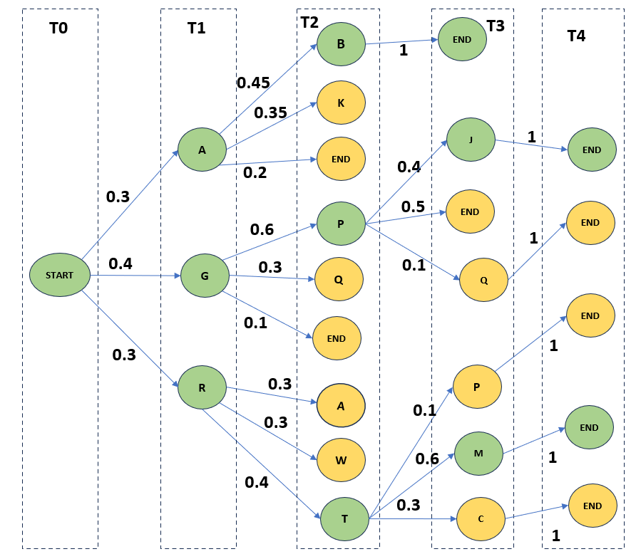
Since the bean width is 3, we’ll generate 3 candidate tokens for next time step. So, at time step T1, we generate three tokens 'A', 'G' and 'R' with probability 0.3, 0.4 and 0.3 respectively. The bean width also dictates at each time step, how many generations will move forward. At time step T1, since we have 3 generation in total which equals the beam width, we consider all 3.

Now, at time step T2, we have in total 9 generations, 3 from each of the previous tokens. But since bean width is 3, we can only move ahead with three sequences. So, at time step T2, we calculate the total probability from root to leaf and select the three with highest probability. We calculate the final sequence probability by multiplying the probabilities of all the nodes used to reach the leaf. For example, for sequence '<START>AB', the final probability is P('<START>' —> 'A') * P('A' —> 'B') which is 0.3 * 0.45 which is 0.135.

Similarly, we calculate the final probability of all the paths from root to the active leaves and pick the top 3 as candidate sequences for further generation.

In our example, those sequences are '<START>GP' followed by '<START>AB' and '<START>RT' with probabilities 0.24, 0.135 and 0.12 respectively.

Note that few paths may end up tied on same score. For simplicity, we resolve this tie by randomly picking the required number of sequences. But there could be more nuanced ways to resolve this tie.

Following the same strategy, the three nodes selected at time step T3 are '<START>AB<END>', '<START>GP<END>' and '<START>GPJ' with probabilities 0.135, 0.12 and 0.096 respectively.

At time step T4, we have reached the '<END>' for all the candidate sequences and we finally pick the sequence '<START>AB<END>' since it has the highest probability of 0.135 among all the generations.

While beam search improves upon greedy decoding, it can still suffer from issues like repetitive texts, it still would not be suitable for an open-ended task like creative writing. This is because more often, the final set of sequences may still be very similar. Beam search also is computationally heavier compared to greedy decoding.

Also, note that since at each time step, we multiply the previous probability by another smaller value, so beam search, which is supposed to generate a sequence with high probability, it kind of favors smaller sequences. There are various ways to alleviate this problem like taking weighted probabilities of the paths, normalizing the probabilities etc. I’ll try to add some references or add a small section here.

‘Diverse Beam Search’ was proposed as an improvement over vanilla beam search. It divides the k most probable sequences into G groups and incorporates a diversity term to maximize intergroup diversity. We’ll not go deeper into this. More details can be found in the paper here.

Contrastive Decoding:

Contrastive decoding intends to push model towards producing more coherent and non-repetitive text, even for long sequences.

Figure 2. From the paper: authors show the outputs generated from greedy decoding, nucleus sampling and contrastive decoding.

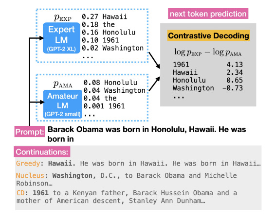
In the figure above, observe how the output from contrastive decoding contains tokens which make the sequence more creative and coherent.

Let’s have a closer look at it.

Contrastive decoding utilizes two LM simultaneously: one big, which is called EXPERT, and the other a small one, which is called AMATEUR.

The key idea: with high chances, the AMATEUR model will be a subset of EXPERT in terms of intelligence and the knowledge space they represent. So, both models would have lot of overlap in terms of making mistakes like repetitions & degenerations, lack of coherence, low quality generation etc. But the EXPERT model will have a distinctive non-overlapping knowledge space and capability representation. If these mistakes are somehow filtered out, mostly the superior capabilities of the EXPERT would remain.

Authors experiment with two sets of models: one where OPT-13B and OPT-6.7B was used as the EXPERT model while OPT-125M was used as AMATEUR. Other set had GPT-2 XL(1.5B) as the EXPERT model while GPT2(100M) base model was the AMATEUR.

For filtering out these mistake modes, authors propose an objective as below:

\(\underset{x_{cont}}{max} \ \mathcal{L_CD}(x_{cont}, x_{pre}) \ subject \ to \ x_i \in \textit{V}_{head} \ (x_{<i}) \ \forall x_i \in x_{cont}\)

• x_pre: the sequence of tokens seen so far, like the prompt or generated tokens

• x_cont: the sequence of tokens generated in current or future time steps

Also note,

• p_EXP: the probability of a token as predicted by EXPERT

• p_AMA: the probability of a token as predicted by AMATEUR

Let’s break it down. It has two components: the CD objective which is subject to a constraint which the authors call Adaptive Plausibility Constraint.

The CD objective is defined as

\(\mathcal{L_CD}(x_{cont}, x_{pre}): \ log \ p_{EXP}(x_{cont}, x_{pre}) \ - \ log \ p_{AMA}(x_{cont}, x_{pre})\)

This objective basically maximizes the log-probability difference between tokens generated by the EXPERT and AMATEUR. It takes into account the log of the probability for the tokens and then picks the token where the difference between the log probabilities is maximum. This rewards the tokens favored by the expert model and penalizes the tokens favored by the smaller model.

For example, in the figure 2 above, we see that both EXPERT and AMATEUR assign relatively higher probability to tokens like 'Hawaii' and 'Honalulu', which results in low difference between the models. However, for the token '1961', AMATEUR assigns much lower score relative to the EXPERT. Thus, the log-prob difference is very high and this token is favored as the next output token. This results in model being more creative while selecting the next token and avoid repetitions.

But this objective alone leads to some false positives and false negatives. The thing is that AMATEUR is still a language model and has learned some representation of the language. This would mean they are not always wrong.

False Negative: They would generate tokens which satisfy some simple aspects of the language like a following ‘is’, ‘the’ etc. and these can get discarded.

False Positive: some implausible tokens, even with lower probabilities for both the EXPERT and AMATEUR, may end up having a significant log difference and thus getting selected.

So, we apply Adaptive Plausibility Constraint, V_head to this objective.

\(\textit{V}_{head} \ (x_{<i}) = \{ x_i \in \textit{V} : p_{EXP}(x_i|x_{<i}) \geq \alpha \ \underset{w}{max} \ p_{EXP} \ p(w|x_{<i}) \}\)

• V_head(x_i) represents the set of candidate tokens for the i-th position in the sequence, given the preceding tokens x_<i, for positions <i

• x_i ∈ V: each element x_i is chosen from the vocabulary set V

• p_EXP(x_i|x_<i): the probability of token x_i appearing as the next token, given the tokens x_<i

• max(p_EXP(w|x_<i): the maximum conditional probability of any element w in the vocabulary set V, given the context x_<i

• α is the parameter that controls the strength of this constraint. Its value is in the range [0,1]

We identify the maximum probability assigned to any token, given the context x_<i and multiply that by α. This becomes the threshold for selecting the candidate tokens. Only the tokens which are above this threshold will be considered as potential candidates for the output as next token.

Note that high value of alpha will result in only high probability tokens being selected while low value will result in chances of lower probability tokens also getting selected.

Consider the false positive case above: the implausible tokens, which will have very low probability as per both EXPERT and AMATEUR, would get filtered from the set of potential candidate tokens due to the threshold applied by this constraint.

In case of false negative, like above, the tokens which should naturally appear as the next output, like "#corn" after "uni" or a "is" or a "the", will have very high probability as per both EXPERT and AMATEUR. But because we have already applied the threshold based on the constraint V_head, the candidate pool of tokens from which we need to select, is itself very small. So, these tokens, even if do not have a very high log-prob difference, will still be competing to be selected as the next output token.

The CD objective and the constraint described above applies to the sequence level. But in actual implementation, this would need to be applied at token level. Authors provide details about how this is factored to token level. They also provide details into how models were selected for the experiments and other ablation studies. Read the paper here.

Figure 3. sample output from the paper

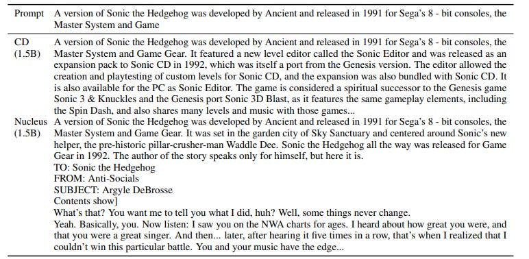
Observe how CD generates more coherent text while nucleus sampling tends to veer away from the actual topic thus making the text incoherent.

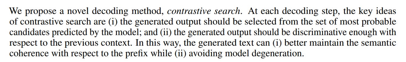
Contrastive Search

Contrastive search was originally introduced in the paper “A Contrastive Framework for Neural Text Generation”. In the paper “Contrastive Search Is What You Need For Neural Text Generation”, authors demonstrate the text-generation capabilities of contrastive search in context of LLMs.

As already seen, methods like greedy approach and beam search tend to degenerate i.e. they start producing often repeating and semantically incoherent and even unrelated text. Contrastive search claims to improve upon that and solve the problem of model degeneration.

Figure 4. Example from the paper 2210.14140.pdf. (Contrastive Search Is What You Need For Neural Text Generation)

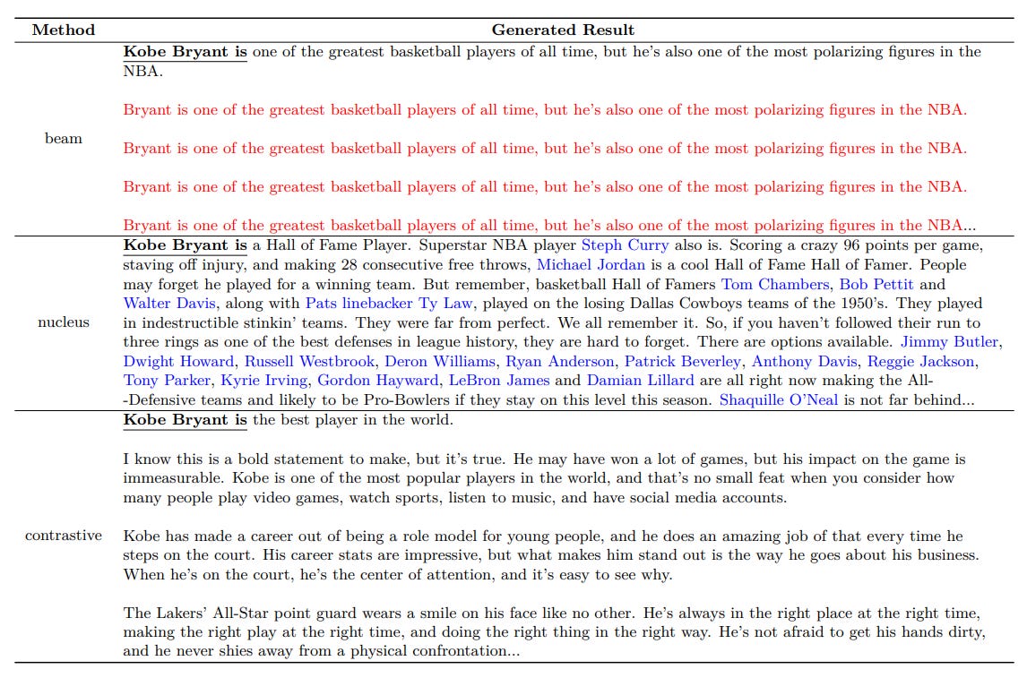
The above examples were generated with the prompt “Kobe Bryant is”. Observe the issues with beam search and nucleus sampling: while beam search produces repetitive text (in red), nucleus sampling quickly veers away from the actual topic (highlighted in blue).

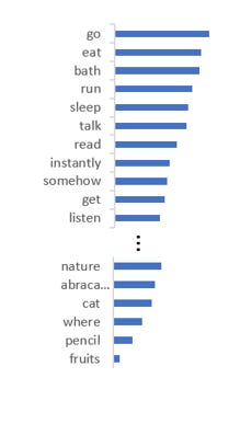
The idea: Use the top-k tokens predicted by the LLM as the candidate set, for the output as next token. Here we are implicitly trusting the model to consider tokens which maintain coherence.

From that set of k tokens, pick the token which minimizes the similarity WRT the previously generated tokens, thus minimizing the chances of repetition while keeping the coherence and context intact.

So, by considering both attributes, contrastive search helps retain the semantic coherence property and reduces the likelihood of model degeneration.

From the paper:

Figure 5. Short description of contrastive search from the paper

To achieve this, the paper introduces a new method to decode the token at timestep t:

• x_t : the token generated at the timestep t

• V^(k) is the set of top-k candidate tokens at the timestep t

• α is a hyperparameter which regulates the impact of penalty

• s(.,.) is similarity function which calculates the similarity between the representation of two tokens. This can be a normal cosine distance calculator.

• h_v : representation of the sequence x_<t + v, as generated by the model

• h_xj : representation of each token x_j, for 1<= j <= t-1

This has two components:

Model Confidence: the probability of the candidate token v given all the token at time step <t. This is the usual sampling from model’s probability distribution p_θ

Degeneration penalty: this is the additional term which helps model avoid generate repetitive tokens. It can be defined as the maximum cosine similarity between the representation of the candidate token v and the tokens in the context seen so far(x_<t).

h_v is computed by the LM given the concatenated sequence x_<t and v.

Then we calculate s(h_v, x₁), s(h_v, x₂) … s(h_v, x_j) and then take a max of these scores which becomes our degeneration penalty. The impact is controlled using α, whose value ranges between [0,1].

So, higher the similarity between the candidate token and the context seen so far, there are high chances the model is heading towards degeneration, thus we impose higher degeneration penalty.

Observe that if alpha=0, this will degrade to normal greedy approach.

---

So, these were some of the deterministic approaches. Let’s see some stochastic ones. These have been making lot of buzz recently, all thanks the shoot up in LLM usage and these are some of the parameters used more often than not to control the generation from these LLMs.

Top-k Sampling

We saw in greedy approach above that the token with the highest probability is selected as the next output token and that can lead to things like repetitions.

So now rather than picking the top token, we can just sample from the entire probability distribution randomly. This gives other probable tokens a fair chance to get selected but then we are increasing the chances of some really bad tokens getting selected as well.

Figure 6. When all the token have a chance of getting selected in random sampling. The prompt being “I was planning to”

To alleviate this problem, we sample only from the set of top k tokens. Simple!!!

Figure 7. We sample randomly but only from the top-k tokens. Here k=7. The prompt being “I was planning to”

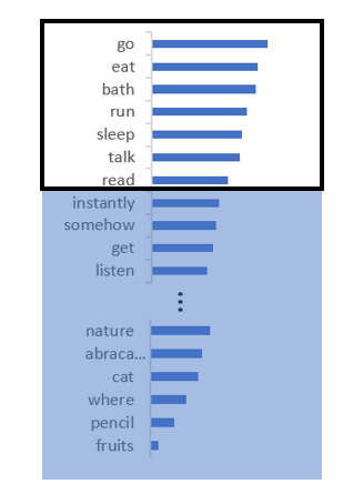
While the idea is very simple, it has its own issues. They suffer from two problems:

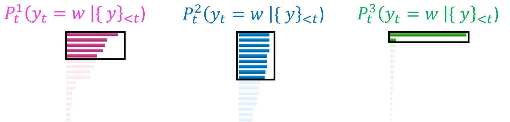
• They can cut-off too quickly which means tokens which could have been a valid output get ignored. This can happen if the probability distribution is relatively flat. For example, in the figure below, ‘read’, ‘buy’ etc. are valid tokens given the prompt “I was planning to” but they get zeroed out because of low value of k.

• Or they cut-off too slowly which means tokens which are totally irrelevant and bad will have a chance of getting selected. This can happen if the probability distribution is peaky. For example, in the figure below, ‘giraffe’ would not be a good token to select, prompt being “I like watching soccer as well as”.

Figure 8. Fast Cut-off and slow Cut-off

These issues illustrate it is hard to pick a good value for k and it becomes a bit of hit-n-trial.

Top-p(nucleus) Sampling:

This method tries to alleviate the problems of top-k sampling. Now, rather than depending on a number k to pick the set of candidate tokens, we rely on probability mass. After all, what we get from the model is a probability distribution over all the tokens in the vocabulary. So, we pick all the token that lie within p% mass of the distribution. This can be said to be equivalent to selecting a dynamic k.

Figure 9. sum of probabilities of minimal set of token greater than or equal to ‘p’. Value of p could be 0.95 meaning select minial set of top token which comprise 95% mass of entire probability distribution.

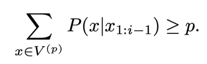
Resulting token sets based on where the mass/nuclei of the distribution is:

Figure 10. Selection based on probability mass, sort of dynamic k in top-k. Source: CS224N.

Temperature Sampling

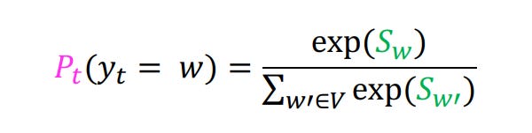
Temperature based sampling is yet another way to introduce randomness to the process of sampling. Recall that the final probability distribution is generated as per the formula:

Figure 11: calculating probability distribution in a LLM

We introduce a parameter τ and divide the logits (i.e. S_w) in the formula above by τ.

So, the new formula becomes:

Figure 12. probability distribution calculation with temperature parameter

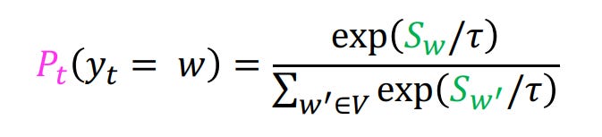
Notice that as the value of τ increases the difference between high logits values and low logit values will decrease. This would impact the eventual softmax scores, thus resulting in a token getting selected which would have been ignored in greedy search. This happens when the value of τ is >1.

However, if the value of τ is <1, the distances between high logits and low logits will be further amplified as will be the eventual softmax scores. So low value of τ will strengthen the dominance of the most likely word.

This is the reason why higher values of temperature will result in more diverse and at times surprising outputs. While lower value of temperature plays it safe, resulting in more predictable output.

A value of 0 for temperature is just greedy search.

Let’s see an example. Suppose the context seen so far is “Sachin is one of the greatest” and we need to select the next word.

In the below table, we have the list of top next words with their corresponding logits, as predicted by model. This is in column 1 and 2.

Figure 13. toy example of effect of temperature on the eventual softmax score

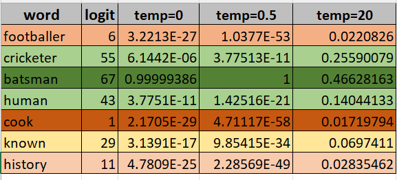
Column 3 is the usual softmax scores based on the logits. Logically, “batsman” has the highest score. “cricketer” and “human” also seem to be a valid completion, thus their logits and softmax in the vicinity of the word “batsman”.

Now when we have temperature=0.5, notice how the difference between the word “batsman” and “cricketer” increased. Other tokens are affected similarly and thus the distribution becomes peakier.

However, when the temperature is set to a high value 20, the eventual softmax scores are much closer. This makes the distribution flatter. So now more tokens would be competing to get accepted as the next output. This results in more diverse outputs which suit tasks like creative writing for example.

Imagine this happening over a much larger set of words, where the vocabulary size is in in the range of thousands. This is why we see the variance in outputs in the recent LLMs when the temperature value is even slightly higher, not even 15 or 20.

What we saw above is a generalized explanation of how temperature affects the generation. In general, the accepted range of temperature for different models is [0,1].

---

This is it for this post. Hopefully, will be writing more to share some learnings. Happy reading and LLMing.

References

• CS 224N from Stanford

• A Contrastive Framework for Neural Text Generation

• Contrastive Search Is What You Need For Neural Text Generation

• Huggingface Contrastive Search Blogpost

• A Thorough Examination of Decoding Methods in the Era of LLMs

• Diverse Beam Search

• Creating Human-like Text with Contrastive Search and GPT-2

• Contrastive Decoding: Open-ended Text Generation as Optimization